This project was carried out by Diana Sarbakysh and Art Moskvin through the Supervised Program in Alignment Research (SPAR), under the supervision of TGT’s Aaron Scher. This analysis serves as a starting point for future work, rather than the final word on this topic: we are fairly confident in the conclusions but less confident about individual details.

Abstract

Verification and confidence-building mechanisms have been proposed to allow AI developers to prove claims about their activities to external parties, such as foreign governments or regulators. AI companies could then claim they are using computer chips for some activities but not others, for instance serving customers but not training new AI models. We examine interconnect limits as a verification mechanism: capping internal network bandwidth in order to prevent large-scale training runs while allowing inference. We prototype this mechanism end-to-end on AI GPUs using both compliant and adversarial workloads, providing a minimal implementation to assist future work. By running multi-modal inference workloads, we also test and alleviate the concern that image or video generation might exceed bandwidth limits: these involve less communication than training. We analyze the pros and cons of this mechanism and conclude that the basic mechanism is straightforward to put in place, and it withstands basic subversion attempts, including the distributed training method DiLoCo. However, there are multiple major downsides of this mechanism, and our prototype lacks realism in various ways. We conclude that network limits are a promising approach to AI verification and confidence-building, and we urge more research and implementation of this mechanism. 

Introduction

Verification mechanisms—processes giving one party confidence another is following agreed-upon rules—are essential for any enforceable international framework to reduce catastrophic risks from advanced AI (Baker et al. 2025, Harack et al. 2025, Scher & Thiergart 2024). A primary goal of such an international framework might be to confirm that new large AI models are not being trained (Scher et al. 2025; Heim and Koessler 2024). One mechanism for such verification is imposing interconnect bandwidth limits between AI accelerators or pods of accelerators. This mechanism operates on the assumption that large-scale training requires sustained, high-bandwidth collective communication across many GPUs, while inference requires markedly lower traffic. This assumption is supported by theoretical analysis (Scher & Thiergart 2024), public evidence about networking for production AI (Patel et al. 2024; Si et al. 2025), and simple experiments in this paper. The primary threat to this assumption is that algorithmic improvements in distributed training could significantly reduce the network footprint of training. 

This report tests interconnect limits end-to-end in somewhat-representative conditions—covering compliant, non-compliant, and adversarial actor scenarios; and provides a complete implementation for further prototyping and red-teaming work. We also discuss the viability of this mechanism, including an analysis of its pros and cons. We encourage future work to develop and implement this mechanism and suggest particular directions for this follow-up work. 

Related Work

While prior work has introduced this mechanism, our report fleshes out minimal implementation and deploys it on hardware. We provide a complete, reproducible MVP and empirical data for researchers and policymakers to build upon.

Chip-use verification. This paper sits within a broader literature on chip-use verification. Various approaches have been proposed to enable AI chip owners to demonstrate to an external party that they are using chips for some purposes but not others (Baker et al. 2025, Harack et al. 2025, Scher & Thiergart 2024). One approach to this problem is to classify chip workloads based on telemetry data (Rahman & Tajdari 2026). Interconnect bandwidth limits are a similar approach to this problem. 

Interconnect bandwidth limits for verification. This mechanism was first introduced by Kulp et al. (2024) under the term Fixed Set, referring to a small set of chips tightly networked together that cannot be easily networked with other chips. Scher & Thiergart (2024) further outline the theoretical basis for bandwidth limiting as a verification mechanism that could block training while allowing inference, and they suggest tentative bandwidth limits based on theoretical calculations. Our work aims to validate the theoretical proof of concept using experiments with AI accelerators. Concurrently with our work, Amodo (2026) prototype tray-level bandwidth limiting using DPUs. The success of their work reinforces the viability of interconnect limits for verification, especially when combined with our empirical results demonstrating that bandwidth limitations differentiate AI training and inference. 

Interconnect limits vs network taps. A similar but more involved approach is network taps (Baker et al. 2025, Cankaya, 2026, Cankaya et al. 2026, Karvonen et al. 2025), which isolate a cluster of chips, intercept the communication to and from those chips, and analyze the information to confirm what chips are doing. Network taps have been prototyped by Ulyssean (2025) and Amodo (2026) using physical taps. Interconnect limits analyze only metadata about communication—specifically, the amount and rate of communication—whereas network taps typically collect and analyze the actual content of communication. For example, a network tap system might involve keeping a log of input tokens sent to a server for LLM inference, their corresponding output tokens, and using another cluster to rerun the workload and confirm the outputs are as expected. 

Egress bandwidth controls for model weight security. Because the weights of a frontier AI model are large (hundreds of GB or more), some have proposed implementing bandwidth limits or monitoring in order to prevent unauthorized exfiltration of AI model weights (Greenblatt 2024). Such limits feature in Anthropic’s ASL 3 security stack (Anthropic 2025). While the use cases are different, work on verification-oriented interconnect limits and model weight security can be mutually beneficial. 

Decentralized and distributed training. Previous research has explored methods of reducing the communication requirements between accelerators for AI training (Prime Intellect 2024, Nous 2026). This work is often called decentralized training or distributed training. DiLoCo (Douillard et al. 2023) is the most salient algorithm for distributed training. It involves individual data-parallel workers conducting a series of local gradient updates (inner steps) and syncing with each other infrequently (e.g., every 100 inner steps). This method significantly reduces the overall communication across an interconnect limit boundary compared to standard data parallel training. Because this algorithm poses a threat to the core assumption behind interconnect bandwidth limits by reducing necessary communication, we use it as an example of an adversarial workload. There are various other methods for distributed training which may decrease communication requirements even further, such as Streaming DiLoCo (Douillard et al. 2025) and SWARM Parallelism (Ryabinin et al. 2023). Distributed training could pose a problem for compute-based AI governance and bandwidth limits, an issue explored with a simulator by Rahman 2026. Rahman investigates whether it would be appropriate to exclude chips from monitoring on the basis that they have internet-grade (not data center-grade) interconnect, whereas we investigate how interconnect could be restricted much more than default and how doing so affects subversion efforts. 

Interconnect bandwidth limit primer

Setup

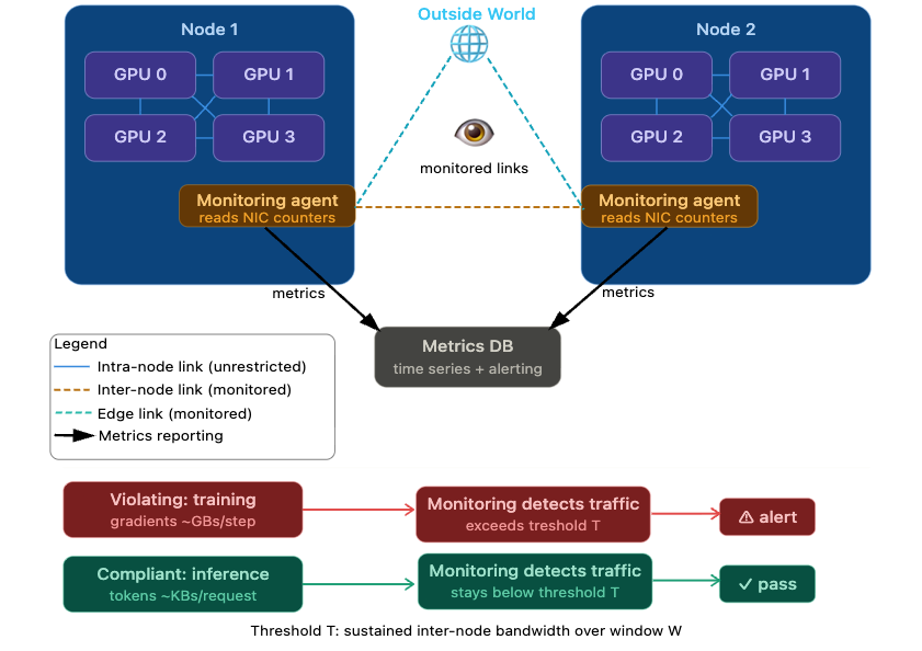
Figure 1 below shows a high-level diagram of a GPU cluster: 2 compute nodes connected together. As part of the governing mechanism, the prover would deploy a special monitoring agent on each compute node and a dedicated server to host a time series database (DB) and alerting stack. The agent exports metrics to the centralized DB, and the alerting tool periodically evaluates the metrics to check if the alert threshold is crossed, in which case an alert is fired through configured channels. The focus is primarily on inter-node communication, though we also measure intra-node communication in this report. 

Core Logic

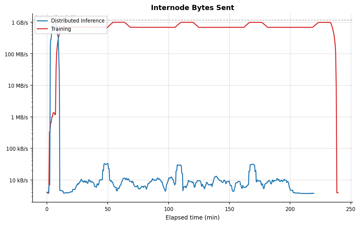
The verification mechanism relies on the currently-true assumption that network bandwidth usage is markedly different between inference and training jobs. Specifically, large-scale pretraining requires more communication between accelerators than inference because training requires synchronizing gradients, whereas inference does not require copies of the model to talk to each other. We demonstrate this assumption using small scale proof of concept workloads on a 2 node cluster (see Figure 2 below).

Both workloads involve significant communication between a small number of accelerators, for instance dozens or low hundreds of accelerators being used for model parallelism (including tensor parallelism, pipeline parallelism, and expert parallelism) or context parallelism (DeepSeek 2025, Yan et al. 2026, Grattafiori 2024). In both cases, a node of accelerators conducts a forward pass over some tokens. In the case of training, each node performs a backward pass to calculate gradients on these tokens and then communicates these gradients to other copies of the model (i.e., other nodes) in an all-reduce communication. For inference, each node receives tokens as input and generates tokens as output, but neither the inputs nor the outputs depend on other nodes. Therefore, each inference node can be isolated or limited from other inference nodes so that it can still conduct inference without being able to efficiently conduct training. 

The difference in communication requirements is enormous. Take, for example DeepSeek-R1, a 671B parameter model. The gradients for such a model would require about 1.342 TB if communicated in BF16, or 1.3e12 bytes, per step, both being sent and received by a node. Step time can range substantially, but 10 seconds is a reasonable order of magnitude, leading to communication requirements of, on average, 2.6e11 bytes/sec; as an approximation, training requires 1e11 bytes/sec. As measured by SemiAnalysis, inference throughput for this model with existing hardware is on the order of 10,000 tokens/sec/GPU or lower, depending on the hardware configuration (Semianalysis 2026). At a reasonable compression of two bytes per token, the required communication an inference node (e.g., of 72 GPUs) needs is therefore on the order of 1.4 MB/s, or 1.4e6 bytes/second; as an approximation, inference requires 1e6 bytes/second. These estimates are imprecise, but they demonstrate why interconnect limits work: inference requires many orders of magnitude less communication between nodes than training. 

Methods

Cluster setup

We conducted experiments on a two-node cluster provided by Azure, each node equipped with 2× NVIDIA A100 80GB PCIe GPUs (160 GB aggregate VRAM per node). We used a PCIe variant of the A100, so intra-node GPU-to-GPU communication traverses the CPU PCIe switch at ~32 GB/s unidirectional, with no NVLink or NVSwitch fabric present. This differs from realistic deployment settings because production training clusters typically use SXM4 A100s (or more advanced accelerators) with NVLink at ~600 GB/s intra-node, so our intra-node bandwidth is roughly 20× lower than a well-provisioned peer.

Inter-node connectivity is a single 100 GbE full-duplex link over plain Ethernet, with no InfiniBand or GPUDirect RDMA.

Full cluster configuration and reproduction instructions are available at github.com/Yayka/ml-infra-profiler.

Workloads

To generate representative traffic we run three categories of workloads, each with variation in architecture and modality, producing a range of communication patterns relevant to the verification mechanism:

1. Violating training runs. We run two training workloads to test whether the mechanism detects unauthorized training across architectural variations. The first fine-tunes Llama 3.1 8B on the C4 dataset for 400 steps, inspired by one of the MLPerf training workloads. Training runs across 2 nodes (4 GPUs total). Each training step triggers inter-node NCCL communication for pipeline-parallel activations and gradient synchronization, making this workload somewhat representative of traffic patterns of large-scale LLM pretraining. The second workload is similar but fine-tunes Mixtral 3.7B, a Mixture-of-Experts (MoE) model.
2. Compliant inference runs. We run three inference workloads across different modalities to establish the bandwidth threshold and verify the mechanism does not generate false positives as inference bandwidth varies. Each experiment generates inference requests at a sustained query rate, measured in queries per second (QPS).

• A base inference run of Llama 2 70B via vLLM on a single node, uses the OpenOrca/GPT-4 instruction-following dataset and generates responses of up to 1,024 tokens per query.
•  A text-to-image inference benchmark uses Stable Diffusion XL. The workload takes short natural-language captions from the COCO val2014 dataset and generates 1024×1024 images.
• A text-to-video inference benchmark takes short action-and-subject captions (e.g. "a person swimming in ocean") from the VBench prompt suite and generates 81-frame, 480×832 videos (~5 seconds at 16 fps) using the Wan2.2-T2V-A14B-Diffusers model.

3. Low communication training (DiLoCo). To test the robustness of the bandwidth limit, we implement a DiLoCo bypass scenario with a much smaller frequency of gradient exchanges (in hopes to run training below our configured limit). The workload trains Llama 3.1 8B on C4 across two nodes in two modes.

• Baseline mode: standard FSDP with full sharding (ZeRO-3) synchronizes gradients across all nodes on every step. 
• DiLoCo mode: each node trains independently using per-node FSDP for a configurable number of inner steps (default: 500), then performs a single cross-node pseudo-gradient all-reduce.

This suite is by no means exhaustive, but covers enough variation in bandwidth consumption to validate the core mechanism and surface early failure modes. 

Monitoring

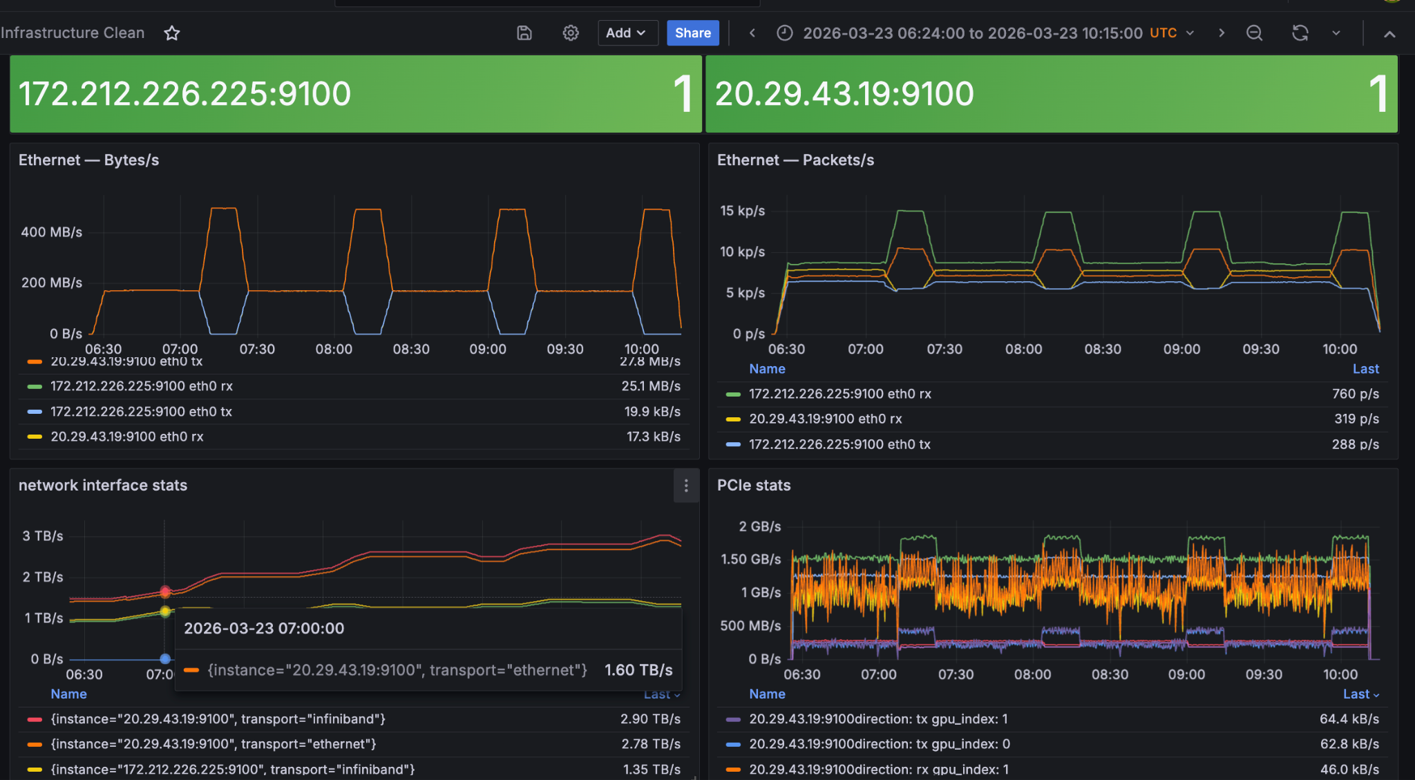
Getting quality network telemetry is the main if not only technical work for this mechanism. We wrote a lightweight monitoring agent and deployed it on each node. All it does is export per-medium network counters to a Prometheus time-series database that we then use to visualize patterns  and reason about good thresholds and signals for the mechanism. For the limited scope of our prototype, the agent tracks four signals: internode bytes sent and received, internode packets sent and received, intranode bytes sent and received (via PCIe counters), and cumulative internode bytes sent. Figure 3 demonstrates these signals during one of the training runs graphed through grafana.

Monitoring precision

Since the quality of the mechanism hinges on the quality of network telemetry reports, we need to discuss precision and limitations of our monitor and its implication.

Sending KB (in case of inference requests) and MB (in case of training all reduce buckets) over Gbps network is a ms if not sub ms latency operation. Hardware counters on the nodes detect these network fluctuations almost instantly, but our monitor only exports these metrics at seconds precision (3 OOM lower precision). So all the fluctuations of the true signal are sampled at the interval of the monitor precision. This is important for instantaneous rates (bytes transferred and packets per second). When we graph these signals, note that we show the averaged values. 

Building a high precision monitor adds non-trivial complexity. It likely involves building a custom solution and achieving ms precision synchronization of time series is likely a separate project of its own. We decided to use the readily available off the shelf metric exporter and timeseries (Prometheus) and the 15 second precision samples it provides is still a meaningful signal for the purpose of prototyping this mechanism, especially when a lot of samples are averaged over a time interval (we use 5 minute averages which considers ~20 samples).

Prototyping Evaluation Protocol

The purpose of this work was to prototype an evaluation protocol and flesh out its details. We define the main steps of such a protocol below (as a first low-cost initial iteration). We then run the above experiments and analyze signal trends to find a meaningful working bandwidth limit and signal thresholds. 

We define two actors:

Prover — the AI-developing org. They own the infrastructure and are responsible for providing reports on network usage. Their obligation is to attest that their systems operate within agreed limits.

Verifier — the auditor. They dictate the compliance threshold, and provide the monitoring tooling, and operate on exported artifacts to confirm compliance.

Step 1: Agreeing on a Bandwidth Limit

The verifier proposes a default inter-node bandwidth threshold. At the time of writing, 1–10 Mbps represents a reasonable upper bound for distinguishing distributed training from inference workloads (see Training Communication Requirements). The prover is expected to accept this default. If the prover can demonstrate that their inference workflows have atypically high inter-node communication requirements, the parties may negotiate a tailored threshold through a back-and-forth.

Step 2: Deployment

Prover instruments their infrastructure using verifier supplied software and instructions:

1. Prover installs the verifier-provided monitoring agent on their infrastructure to export inter-node communication metrics.
2. Prover configures the reporting pipeline — live dashboard, periodic reports, or both — according to the verifier's specification, including scrape interval and report frequency.
3. The prover attests that the exported metrics are accurate and complete. The strength of this attestation can vary depending on the trust model:
   
   • Minimal: Trust-based attestation — the prover asserts compliance without independent verification.
   • Stronger: Hardware-based attestation (e.g., TPM or TEE) providing cryptographic guarantees.
4. Regardless of method, the attestation must cover two core claims: (a) the monitoring agent accounts for all inter-node links, and (b) the reported metrics have not been tampered with.

Step 3: Verification

The verifier accesses the dashboards or saved reports and checks if the network signals remain below the agreed thresholds across all node pairs. If so, the verifier considers the prover compliant.

Results

Proposed bandwidth limit and thresholds

Based on the experiments, following thresholds work for our setup—specific to the models and cluster:

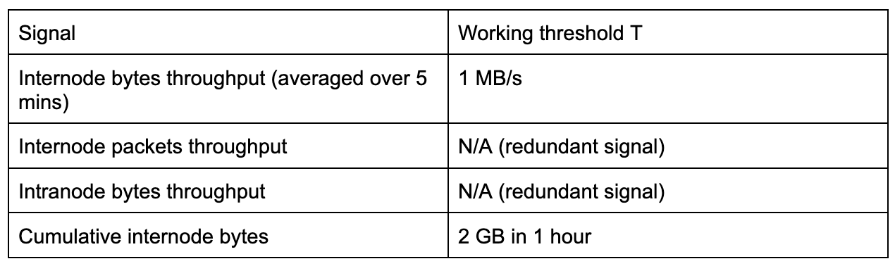
The above thresholds would alert us on non compliant workloads. If we were to go beyond alerting, and set a hard limit on internode bandwidth, 1MB/s limit prevents violating training runs to complete in a reasonable time.

Inference vs. Training

To evaluate the interconnect bandwidth limit against unauthorized training, we simulated a violating actor attempting to run full-scale distributed training across the cluster. We tested two distinct paradigms to confirm the detection mechanism generalizes: a dense transformer (Llama 3.1 8B) and a sparse Mixture-of-Experts (Mixtral 3.7B MoE).

Both training workloads utilized Fully Sharded Data Parallel (FSDP) with a FULL_SHARD strategy (ZeRO-3). In this setup, every forward pass triggers an all-gather of parameters across all nodes, and every backward pass triggers a reduce-scatter of gradients.

As expected, standard FSDP training requires massive, continuous synchronization between nodes. The telemetry data (shown in Figure 4) reveals a stark contrast to inference. Both the dense and sparse training runs reach averaged internode communication from 2 GB/s to 3 GB/s. 

Note that the training lines (green and red) for internode bytes and packets appear as flat lines at around 2 GB/s and ~100k p/s instead of sawtooth, due to the low sampling rate. The true signal would be a series of spikes hitting near-line-rate, and the flat line we see is just the time-averaged value of many rapid I/O bursts per scrape window.

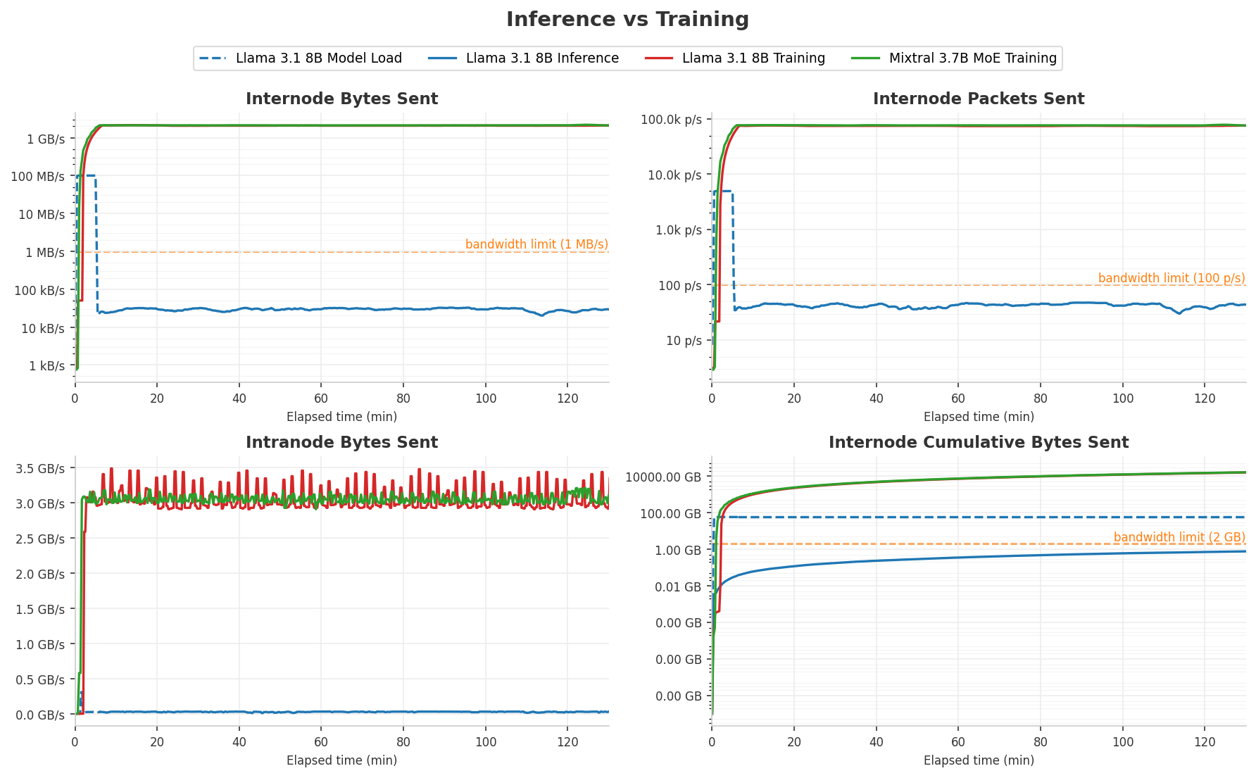
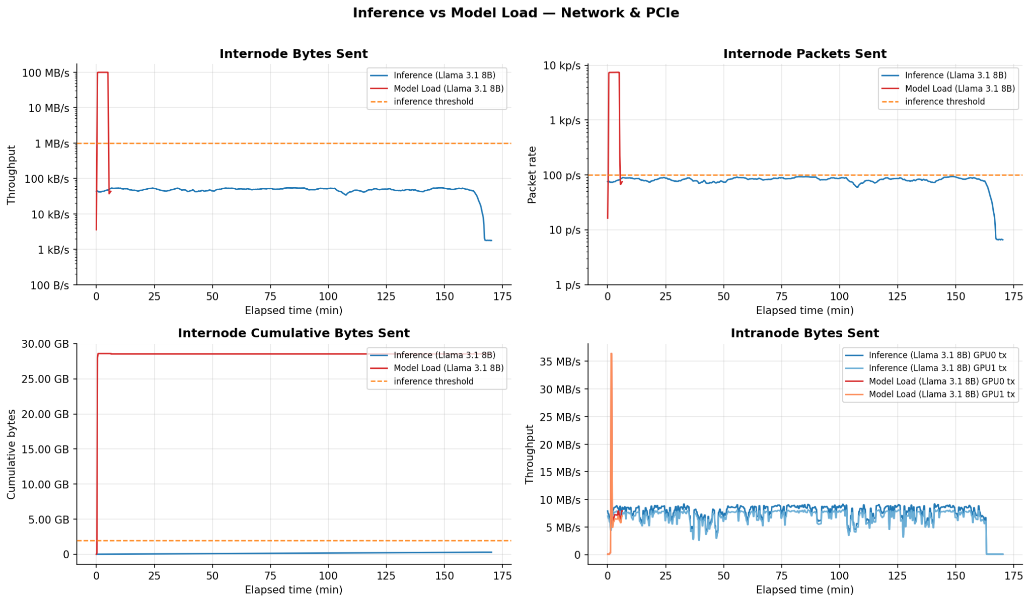
Figure 5 shows a demonstration of what a complying actor’s network traffic would look like. While main inference traffic (blue) is small (well below the limit), to run the inference workflow, the model first needs to be loaded onto GPUs, and this model load operation rises above the strict 1MB/s limit. There are various potential solutions to this issue, and we discuss them in the discussion section.

Multimodal Inference

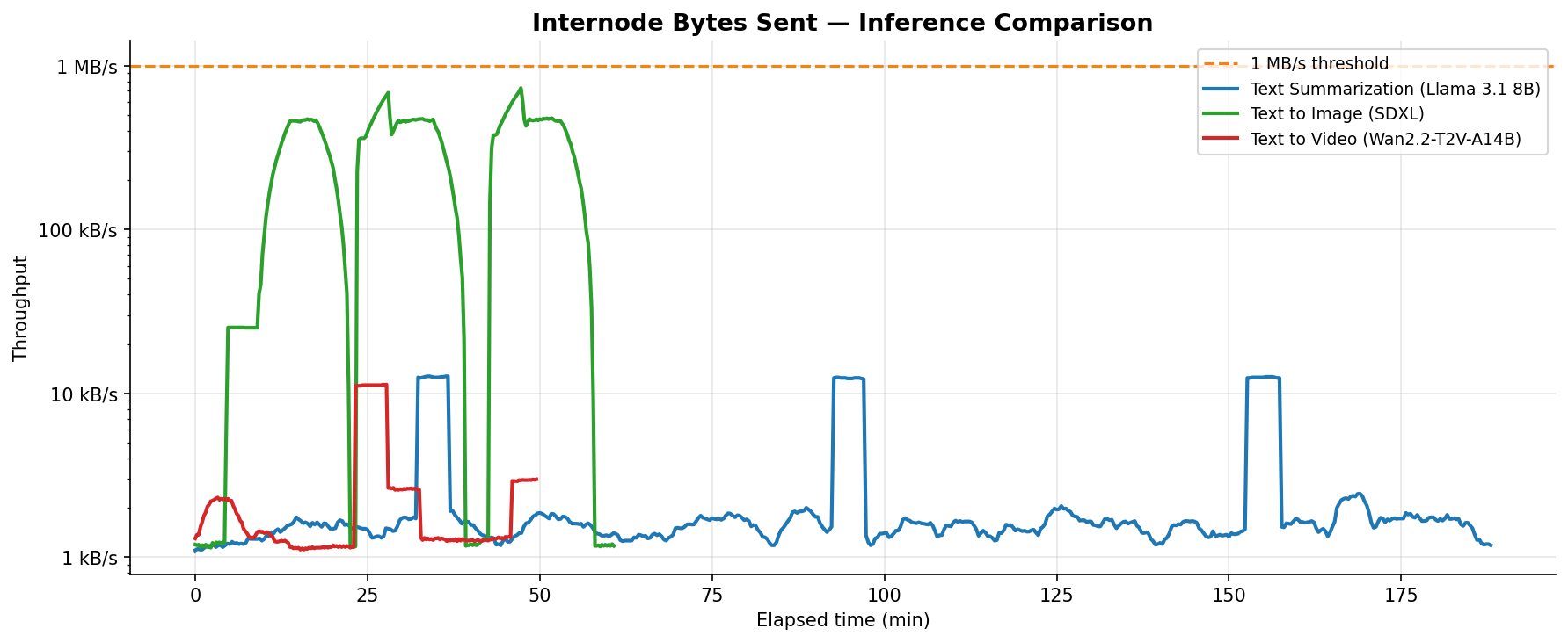
We ran inference jobs with different modalities (i.e. in addition to text summarization workloads, we ran text to image and text to video generation workloads) to see if notable differences in  traffic patterns arise. While generation speed and size of sent content varies, the general pattern stays the same: bursty with predictable peaks. In real deployment, this means limits should ideally be tightly tailored to the nature of inference workloads run on a cluster, taking into consideration queries per second (QPS) and the size of generated content. For instance, in Figure 6 we see that 0.5 QPS with ~500 word response length, text summarization workload stays well below the limit, while 1024x1024 image generation at the same QPS has peaks of 700KB/s approaching the 1MB/s limit. In contrast, short video generation workloads are more compute intensive, so they have longer stretches between bursts and less communication. 

Low Communication Training

To imitate a malicious actor trying to evade detection, we ran Llama 3.1 8B training using the DiLoCo (Distributed Low-Communication) optimization. The DiLoCo run utilized a 2D FSDP device mesh that restricted all-gather and reduce-scatter communications to remain purely intra-node. Cross-node communication was restricted to periodic pseudo-gradient averaging, configured to sync every 500 inner steps.

As expected, Figure 7 shows that the DiLoCo optimization successfully reduced the cross-node traffic footprint while preserving training progress. Total internode data transferred dropped by two orders of magnitude, from over 10 TB in the baseline run to approximately 100 GB. Bandwidth rate also changed its pattern – the continuous 2 GB/s stream seen in the baseline was replaced by no traffic with occasional synchronization spikes reaching roughly 0.15 to 0.20 GB/s.

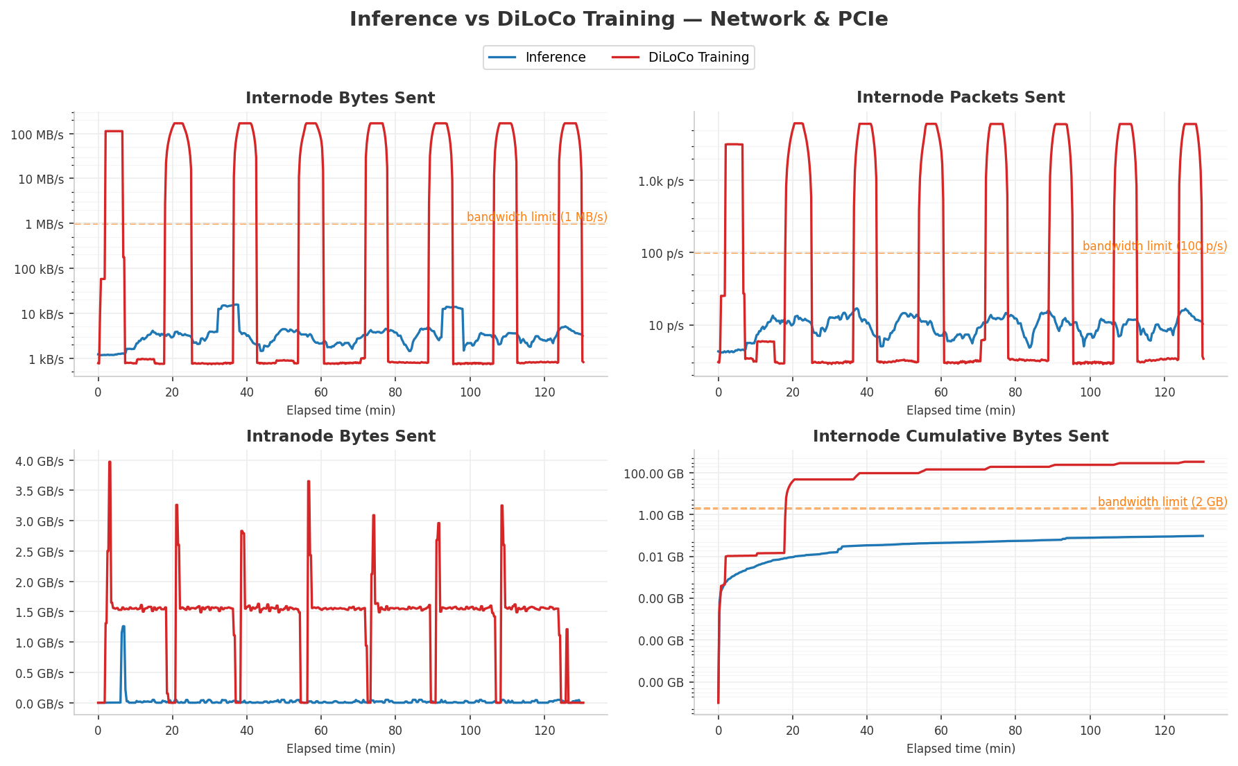
Despite this massive reduction in overall communication, our detection mechanism successfully detected the “sneaky” workflow. Even with DiLoCo syncing every 500 steps, the regular spikes of hundreds of MB/s are vastly distinguishable from inference traffic operating at roughly 10 KB/s as shown above. Consequently, our alerting rule configured to flag durable bursts over a low threshold (e.g. 1 MB/s) easily catches the optimized distributed training approach.

Discussion

Pros and Cons analysis

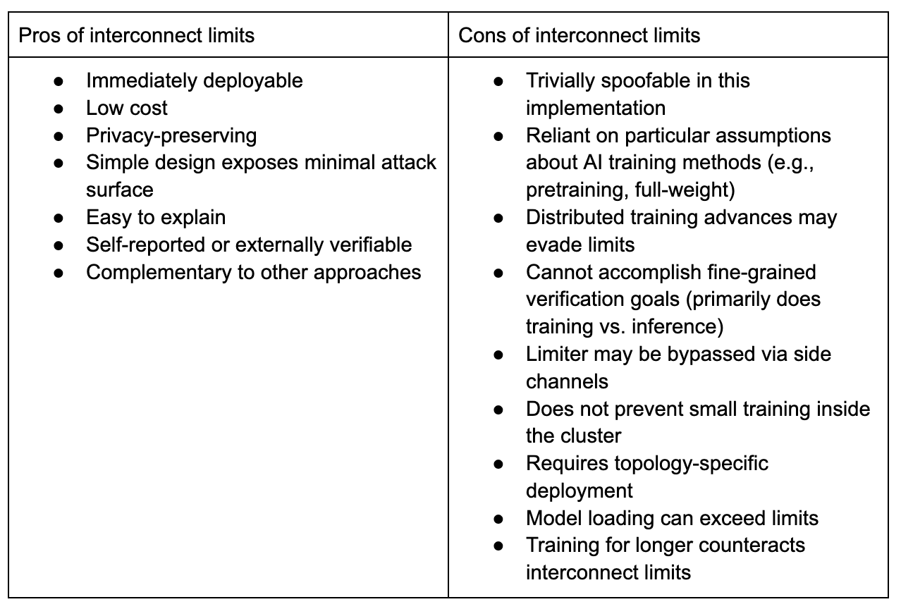
Pros of interconnect limits

• Immediately deployable. Simple software monitors and limiters can be deployed with small investment from the engineering team (on a scale of a couple person weeks). Monitor and limiters are designed to be easily retrofittable with minimal assumptions on underlying hardware and software ecosystems, so can be deployed without modifying core code.
• Low cost. Compared to hardware based verification mechanisms, software based monitors and limiters shouldn’t require any capital expenses. 
• Privacy-preserving. Network traffic reports of bandwidth size and flows do not disclose PII or sensitive company data. Depending on who the information is accessible to, it could leak some information about the AI models running, but this risk could be mitigated easily. All information passing through a bandwidth limiter could be encrypted. 
• Simple design exposes minimal attack surface. The mechanism is simple, minimizing both the attack surface for adversaries and the potential for critical implementation mistakes. 
• Easy to explain. This mechanism is straightforward and does not require a technical background to understand: the trust assumptions are minimal. This may be useful for garnering public support, raising political will, and convincing relevant stakeholders to use the mechanism. 
• Self-reported or externally verifiable. Organizations can initially implement this mechanism as a voluntary measure, and then later regulation could require it, and enforcement could be verified by external parties. The mechanism is flexible along this dimension and would make sense, from a cost-benefit perspective, in both cases. 
• Complementary to other approaches. The mechanism can be paired with chip-level reporting, other telemetry data, and many other chip-use classification methods. It does not prevent the use of these other mechanisms or get in their way. 

Cons of interconnect limits

• Trivially spoofable in this implementation. In our software-only implementation, this mechanism runs the prover’s software on the prover’s hardware, giving the prover control over the entire measurement and reporting pipeline. 
• Reliant on particular assumptions about AI training methods (e.g., pretraining, full-weight). The interconnect differences between training and inference are primarily true for full weight pre-training. By contrast, reinforcement learning (RL) involves performing a large amount of inference paired with a small amount of traditional “training”. Another method that deviates from this norm is LoRA, training a small fraction of weights and thus involving less inter-node traffic. We leave a full analysis of whether interconnect limits would prevent these methods for future work but note that the overall mechanism may not be effective given such methods. 
• Distributed training advances may evade limits. Current distributed training methods are still differentiated from inference, but further advances in distributed training may enable training below the limits. 
• Cannot accomplish fine-grained verification goals (training vs. inference primarily). This method is useful for differentiating inference and training, but it is unable to accomplish many verification goals such as differentiating inference between two different models. 
• Limiter may be bypassed via side channels. The limiter would work by default on known communication channels, but there may be other communication channels, including ones that are hard to detect (e.g., physical side channels). 
• Does not prevent small training inside the cluster. If AI training could take place within a cluster, not crossing interconnect limits, the limits would not prevent this training. 
• Requires topology-specific deployment. The specific implementation of this mechanism depends somewhat on the topology of the hardware, so a small amount of customization is needed. 
• Model loading can exceed limits. Within inference workloads, some activities exceed the interconnect limits, such as the initial phase where the model is loaded onto the cluster. This is a small problem, fixable, for instance, by looking at aggregate bandwidth over time, carving out exceptions for infrequent bursts of communication, or implementing a trusted process for allowing certain communication above the bandwidth limits (e.g., model weight are first loaded onto a verifier-trusted server, analyzed to confirm they are allowed to be sent to the cluster, and then sent into the cluster). Model weight loads are also a one-directional transfer, different from training. 
• Training for longer counteracts interconnect limits. If interconnect limits are in place, an adversary could train for longer, using lower throughput but making up for it with more wall clock time, to reach the same total compute. This is not a major concern because reasonable limits would slow training by a prohibitive amount, e.g., 100x. 

Limitations of this analysis

There are numerous limitations of our experiments that affect their relevance to production clusters. 

• Non-realistic cluster. We demonstrate a proof of concept using just four GPUs across two nodes. Production inference clusters often use dozens of GPUs spread across many nodes (DeepSeek 2025). 
• Small models with limited types of parallelism. Our experiments use small models that fit on either a single GPU or two GPUs. Production inference clusters often use multiple types of parallelism simultaneously, which could lead to different results in the efficacy of interconnect limits. 
• Non-production AI workloads excluded. We consider standard training and inference workloads based largely on MLPerf; however, some workloads would not be nicely categorized into these types. For example, a significant amount of chip use is experimentation (Denain and Wu 2025), not final training runs, and this chip use may involve workloads that look different to production training or production inference. Similarly, we do not test non-AI uses of AI-accelerators, such as weather simulation. 
• Other external validity issues. Principally in this work, we run experiments in a controlled setting, not passive monitoring of real data center use. There are many potential differences between our setup and that of production systems. For example, we don’t use nor take into account inference optimizations like KV caching. 
• Alerts can only be as sensitive as the monitor. Our monitor only samples at 15 seconds intervals, and alerts evaluate on data exposed by the monitor. E.g. current alerting only triggers if throughput goes beyond 1MBps at the end of the sampling period. So alerts cannot trigger instantaneous throughput, or anything sooner than 15 seconds sampling rate. This is also a security issue, since an adversary could set up their violating workflow to run in between the sampling window, and never trigger the alert this way (until the 2GB per 1 hour limit is hit, in which case cumulative bytes alert fires). To increase sensitivity of alerts, you would need to improve the precision of the monitor. But making sub millisecond high precision monitors and reporting pipeline is, from our experience, a non trivial task and can significantly raise the cost of adoption. Alerting on averaged rate (as opposed to instantaneous rate) still works. But generally, alerts based on instantaneous rates are noisy, and it is much more reliable to alert on volume of traffic transferred (2GB over 1 hour period in our case). Note that the proposed threshold of 1 MBps still works as a hard bandwidth limit, and imprecise sampling does not pose an issue here.
• Our monitor is not complete. For this prototype, we only monitor channels where we produce traffic: main ethernet NIC and PCIe. An exhaustive network footprint monitor would capture all of the layers: all physical nics and management networks.  
• Training workflows’ gradient all-reduce operations complete in milliseconds, so our figures do not show a precise communication pattern of training runs.

Future directions

Our work is only initial proof of concept for the verification mechanism, serving to confirm this approach is technically viable with no major issues. However, for an overarching goal of deploying and relying on this mechanism for coordination, much work is needed to “productionalize” it. Below we outline our vision of such work to get us closer to deployment in order or priority. 

Run on representative hardware. We had to make tradeoffs in hardware to get the setup for experiments run: we used cheaper A100 nodes instead of Hopper series, GPUs were connected via PCIe and nodes were connected by regular Ethernet. While we expect experiment re-runs on a better setup to produce similar results, it is a low-effort extension of our work that would win this approach good credibility that would take us closer to real world deployment.

Basic red-teaming. This report barely touches on security. We only demonstrated a naive bypass attempt that fails with basic DiLoCo, but the overall robustness of the approach is still under question. While we relax security requirements in favor of accessible adoption of this method as a confidence building measure within a single country, our implementation is not viable for production. For one, monitoring and limiting is implemented purely in software and we lack any measures to verify that the prover is reporting accurate traffic data. It wouldn’t take much effort from an average developer to mask failures, let alone from a state level attacker. It is critical to develop more secure implementations.

Identify practical worst case scenarios. This mechanism relies on a key assumption that inference produces markedly (orders of magnitude) smaller traffic footprint. A big unknown is whether production training or inference cases exist that break this assumption. And if so, how dangerous would it be to ignore them. We only ran basic variations of inference workflows (text to text, text to image, text to video) and from this limited data extrapolated that production inference load still produces traffic distinguishable from training. But production inference could look different at frontier labs and could have a larger traffic footprint. Similarly, we only ran basic implementation of DiLoCo training, and we don’t know if a dangerous training run can be achieved with substantially less internode traffic. Clarifying this unknown is the next step at derisking. Identifying worst-case scenarios could also investigate whether RL post-training bypasses interconnect limits and results in significant capability gains. Investigation should also assess the viability of LoRA pre-training and other methods that might collapse the communication differences between training and inference. 

Test with more varied workloads. Related to the above point, it would be good to test and confirm if all major production variations of training and inference produce similar/comparable traffic footprint. 

Process for defining a good limit. As with any alert, the stricter the bandwidth threshold used,  the more robust this mechanism is, but if it's too low we run the risk of false positives. We primarily used experiment run results and rough visual cues from related graphs to come up with a bandwidth threshold. This will not produce the most accurate threshold and it requires actually running all variations of workloads for prolonged time to identify trends. If limits can be calculated accurately without workload run, this would significantly simplify the mechanism and make adoption easier.