This project was conducted as part of MIRI Technical Governance Fellowship and was authored solely by Fernando Ruiloba Portilla; the project was mentored by Peter Barnett. It does not necessarily reflect the views of the organization.

Summary

MIRI's Technical Governance Team recently proposed an international agreement to halt the development of superintelligence until it can be done safely. At the heart of the proposal sit three compute thresholds: a Strict Threshold at 10²⁴ FLOPs, above which training runs would be prohibited; a Monitored Threshold at 10²² FLOPs, above which training runs require declaration, approval, and oversight; and a Post-training Threshold at 10²³ FLOPs above which post-training runs would be prohibited.

One concern is that, as AI technology improves, it may become possible to build a dangerous model that significantly improves capabilities without using extra training compute, effectively bypassing MIRI’s pre-training compute thresholds by weakening the correlation between pre-training FLOPs and model capabilities (the infamous scaling laws).

This post analyzes inference scaling, one such mechanism threatening training compute thresholds. It studies two ways in which inference scaling could undermine training compute thresholds, previously explained by Toby Ord. First, by simply increasing model capabilities after model deployment and second, by recursively generating high quality synthetic data used for training a superior model, a form of recursive self-improvement.

On the first concern, the data suggests inference scaling does not completely break the thresholds. Inference scaling has diminishing returns, and performance plateaus past a certain number of tokens in every release period I observe. Models trained with more compute reach higher scores at any inference budget, so top performance still requires both training and inference scaling. Saving 1 OOM of training compute costs roughly 1.4 OOM of inference compute, in line with Villalobos and Atkinson. The substitution is also uneven across tasks, with larger models gaining more capability per inference token on harder, longer-horizon tasks and smaller models benefiting more on easier ones. Over time the curves shift upward and the maximum useful token budget grows, while the rate of gain per token shows no consistent trend.

On the second concern, the evidence is more circumstantial but harder to dismiss. Models are consistently smaller and more overtrained than Chinchilla-optimal; AI labs choose this configuration when optimizing for cheap inference. The cost to run evaluations is also falling sharply, about 73x per year on the Artificial Analysis Intelligence Index. Together these trends collapse the marginal cost of producing high quality reasoning traces for post-training, putting the preconditions for this type of recursive self-improvement in place even though the loop itself is not directly observable in the data.

Reasoning models

In late 2024, OpenAI released a new type of model, a “reasoning” model that spends more time “thinking” before responding. Reasoning models allocate additional compute at inference time to generate chains of reasoning. This chain of thought helps the model break down complex tasks, recognize its own mistakes, and correct its strategies before providing an answer. On certain benchmarks (GPQA, MATH, and Mock AIME), reasoning models achieved a 10x compute equivalent gain (CEG), meaning a non-reasoning model of similar scale would need 10 times more training compute to match the same level of performance.

Inference scaling for deployment

This leads us to Toby Ord’s first argument for how scaling inference could “derail the current paradigm of AI governance via training compute thresholds”. This argument basically boils down to: if scaling inference gets you more capabilities at a lower cost compared with pre-training, then we can just redirect our compute resources towards inference, making training compute less relevant. My intuition is that it doesn’t work like that, so I decided to perform some data analysis.

Inference scaling has decreasing returns

It would be worrisome for training compute thresholds if we could just keep scaling inference compute and keep getting better results. The reality is that inference scaling has diminishing returns, and performance plateaus past a certain number of tokens.

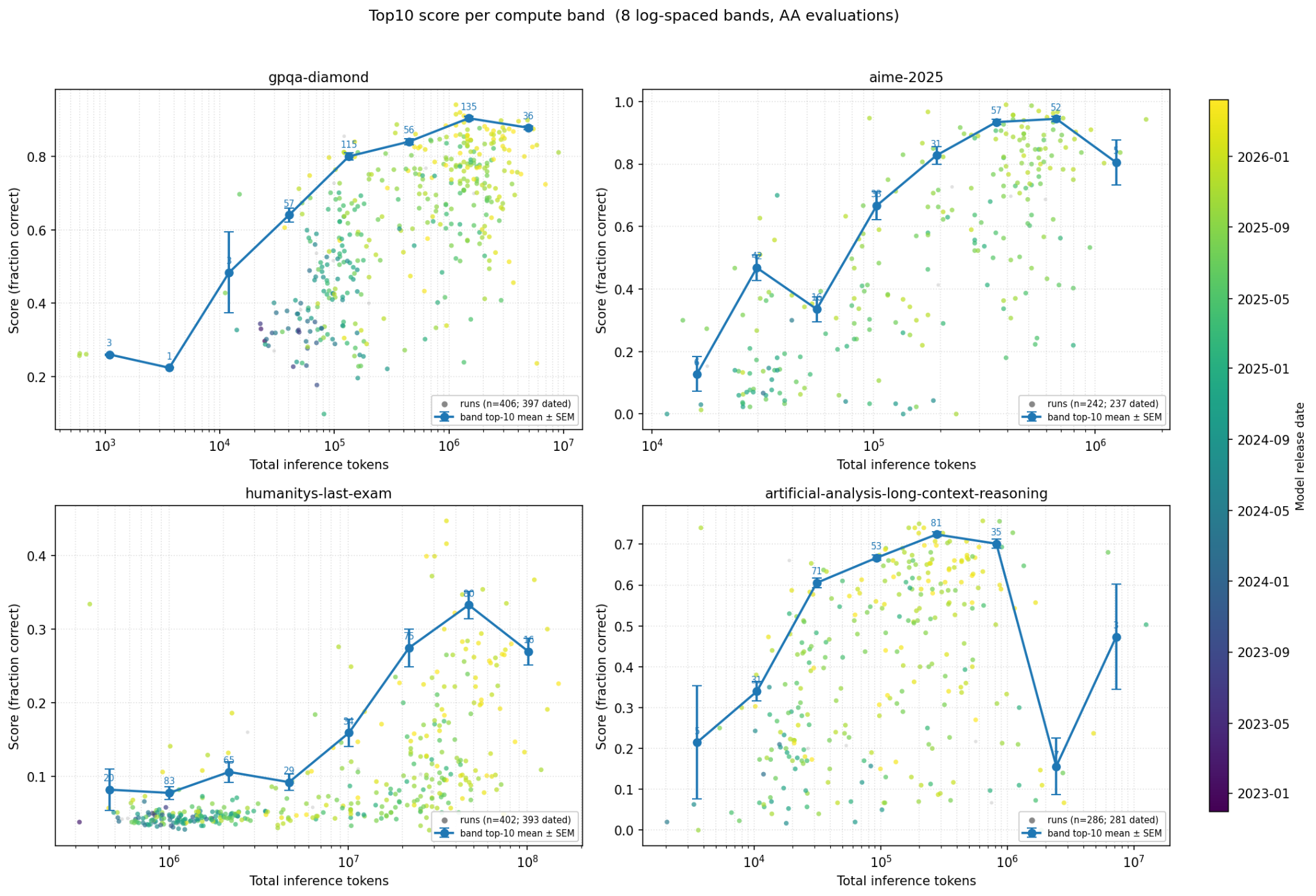
The graph above plots model scores in different benchmarks against the number of inference tokens used to reach that score. Each model is represented as a colored circle, where the color represents the model release date. The graph also draws a trend line over the average score for the top-10 models for each inference token budget.

The trend-line shows the decreasing returns behavior. The graph also shows that some models achieve much higher performance than others for the same inference token budget. Another aspect is that newer models tend to score higher across benchmarks and can use more inference tokens.

Total capabilities are still bounded by training compute

While inference scaling might sometimes generate larger performance gains for less compute than scaling training compute, data analysis suggests that models using a bigger amount of training compute still yield higher performance at any given inference token budget. As I suspected, top performance requires both training and inference scaling.

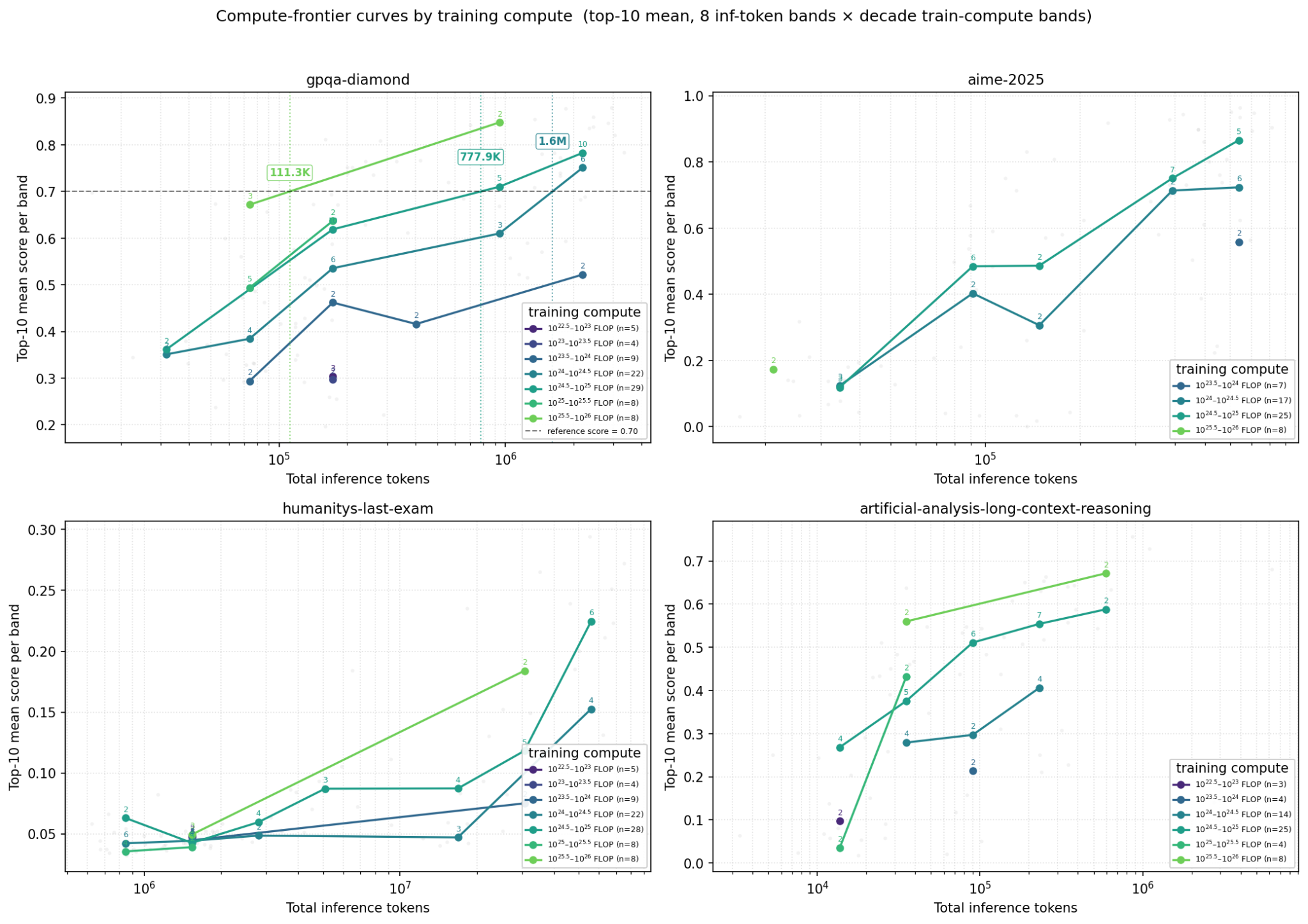
While they weren’t explicitly talking about reasoning models, Villalobos and Atkinson explained the relationship between training and inference compute. They estimated that it was possible to increase the amount of inference compute by 1-2 orders of magnitude (OOM), in exchange for saving ~1 OOM in training compute while maintaining similar performance. In Figure 2, we can see that in order to get the same GPQA-diamond score as a 10e25 model, a 10e24 model needs to use 1.6M inference tokens, which is 1.4 OOM more than the 10e25 model (111.3k inference tokens). This is in line with Villalobos and Atkinson’s estimations.

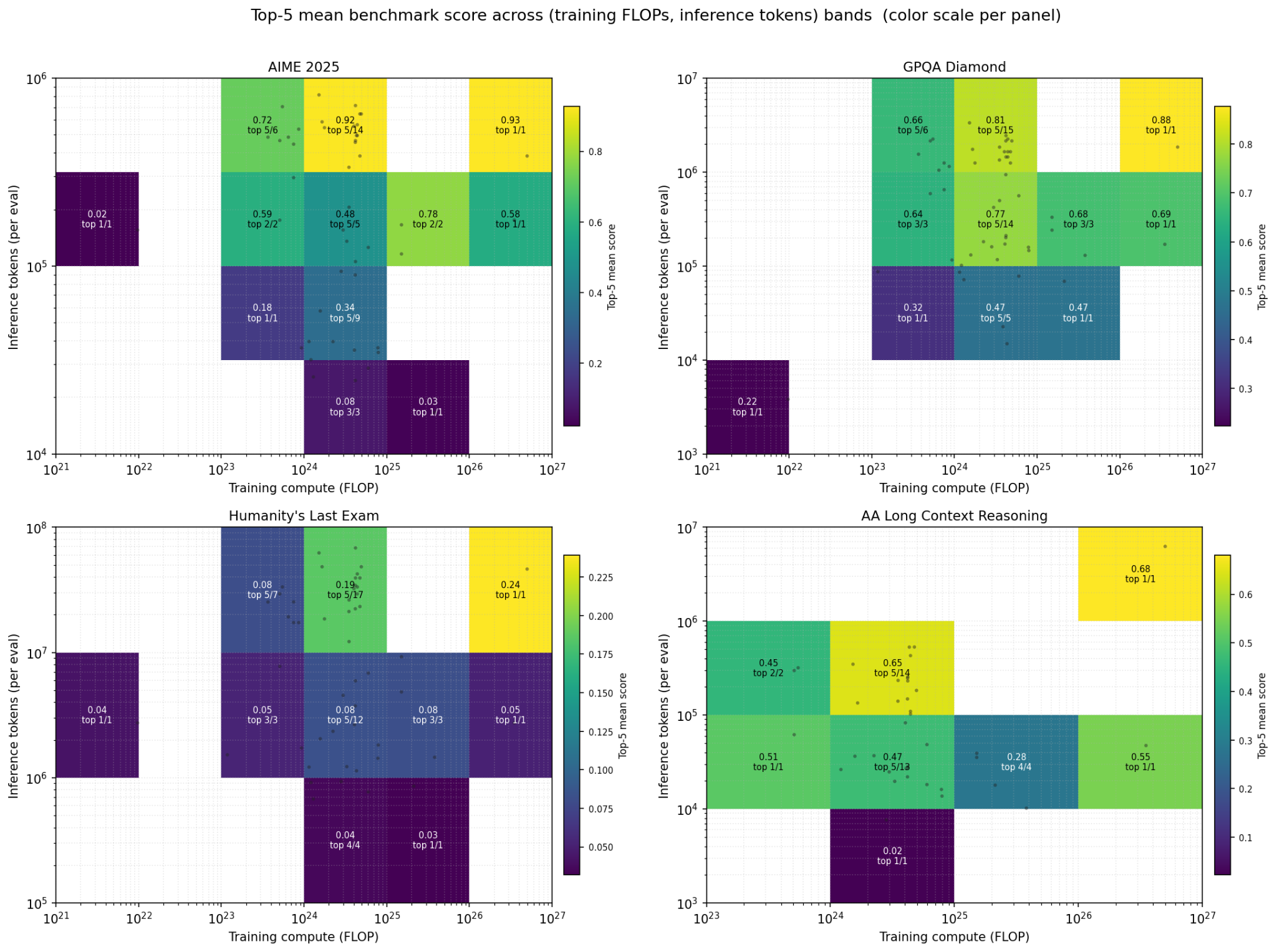
This trade-off has limits, of course. We saw that scaling inference beyond a certain threshold for a given training compute doesn’t yield any more results. In Villalobos and Atkinson’s post the opposite is also true: scaling training indefinitely without scaling inference leads to a diminishing returns in capabilities. They depict this relationship as L-shaped iso-capability curves, where the trade-off is effective at certain inference/training budgets. Figure 3 shows the top-5 mean scores across benchmarks, binned by training compute and inference tokens. Even with limited data, we can start to trace the L-shaped iso-capability curves for different amounts of training compute and inference tokens. Take AA Long Context Reasoning, for example: models trained with 1e23-1e24 FLOPS needed one OOM more inference tokens to reach the same score as models trained with 1e24-1e25 FLOPs.

Inference scaling efficiency varies across tasks

Villalobos and Atkinson’s trade-off rule is helpful for understanding the relationship between training and inference compute. However, the reality might be a little more nuanced. Figure 4 shows the inference scaling behavior for two models, gpt-oss-20b and gpt-oss-120b. They were both released on the same date but differ in their number of parameters (21B total / 3.6B active vs 117B total / 5.1B active) and the amount of compute used to train each of them (the 120B model used 9x more training compute).

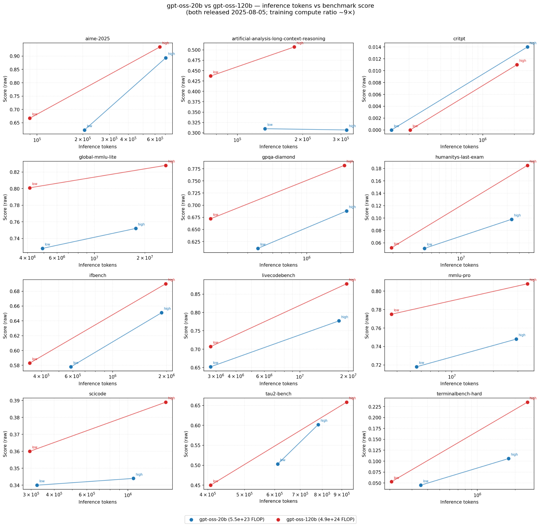
Usually, for both models, the score increases as we scale the inference token budget. However, we can see some crucial differences. First, the bigger model gets better scores across all inference token budgets. Second, and more interestingly, the score increases at different rates depending on both the model size and the benchmark. This result is something Ord already suspected: that scaling inference is much more useful for some tasks than others. Villalobos and Atkinson also theorized about different tradeoff rules for different types of tasks.

To better compare the differences in inference scaling behavior, Figure 5 plots the ratio between the slope of the bigger model and the smaller one. It shows that, for the SciCode benchmark, the bigger model is able to get 5.15 times more performance per additional inference token than the smaller model. On the other hand, the smaller model derives more capability gains per inference token used than the bigger one on tau2-bench.

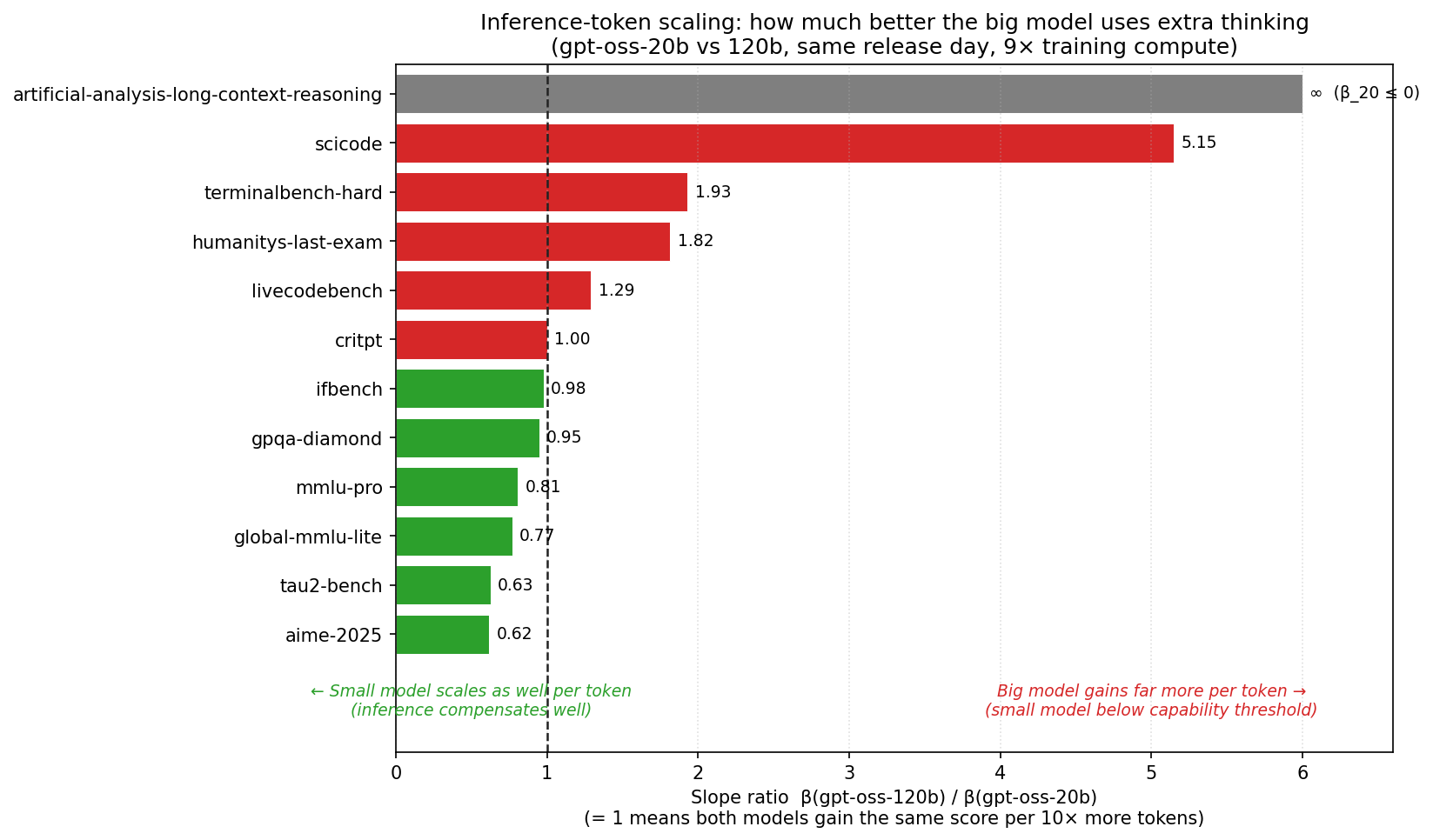
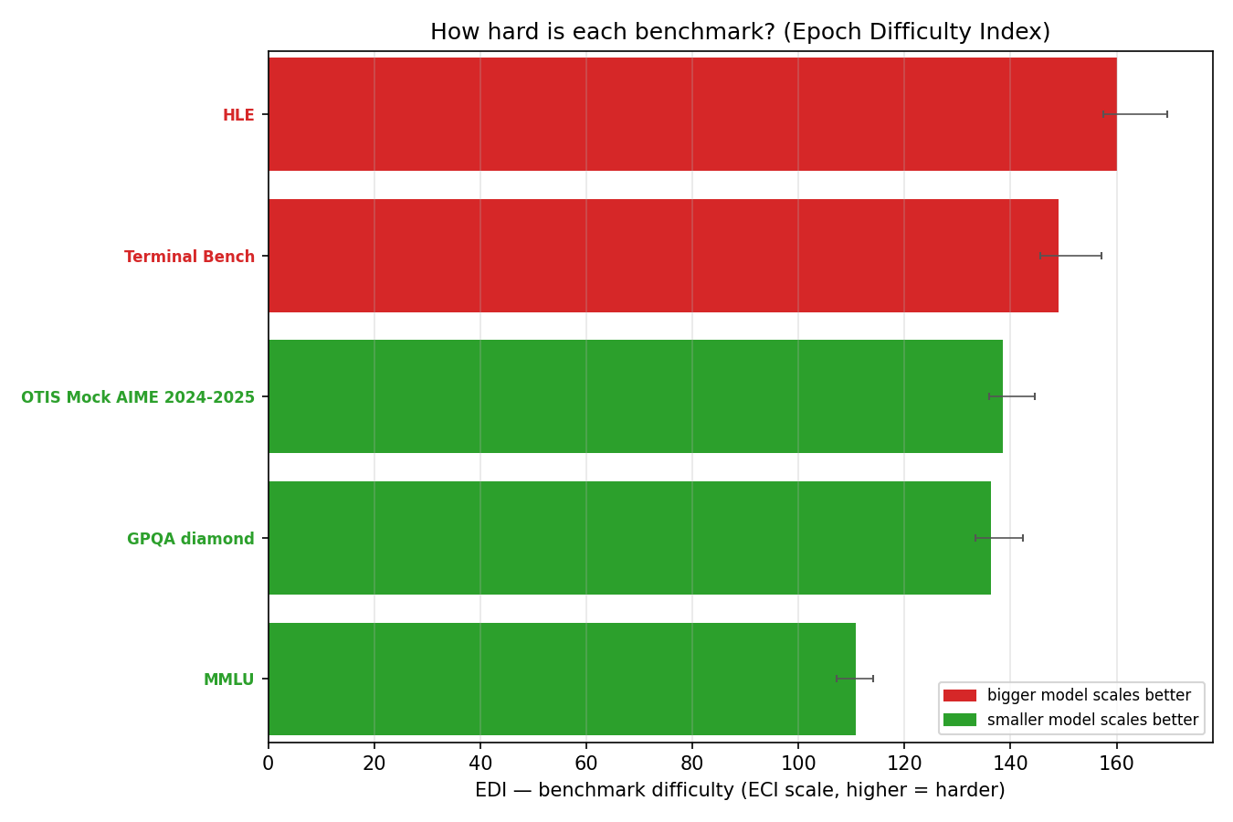
A plausible reason is that the problems are tractable enough for the smaller model to score well without any further scaling. Figure 6 shows the difficulty level for each benchmark based on their Epoch Difficulty Index. While the order is not exactly the same as the graph above, we can see that the bigger model with more training compute scales better against the harder benchmarks. There might be a correlation as well with the length of the tasks that each benchmark requires. Larger models are known for performing better in tasks with longer task horizons.

Inference scaling over time

So far, there is evidence that inference scaling is still dependent on the amount of training compute, meaning that training compute thresholds remain a valuable tool for AI governance. This relationship could erode over time, however, undermining the case for thresholds. I decided to perform more data analysis to understand how this relationship has changed over time.

Diminishing returns are persistent across time

A true source of worry would be whether diminishing returns are becoming “less diminishing”. This would mean that we could scale inference indefinitely and keep obtaining capability gains.

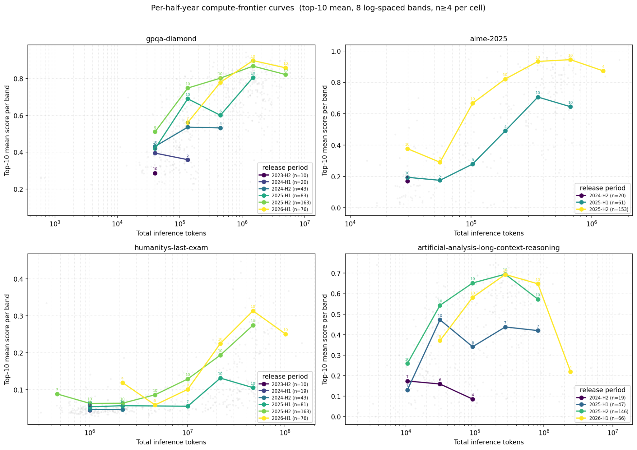
To see whether the diminishing returns behavior has changed, I performed naive data analysis by plotting the mean score from the top 10 models across different inference token budgets for different periods of time. This plot is shown in Figure 7. It shows how the curves are moving upwards, meaning that models are getting more performance for the same number of inference tokens. However, all periods still display diminishing returns. For now, there is no sign of infinite gains through unbounded inference scaling.

Inference scaling is getting more efficient and is able to get returns for longer

We saw that the curves shift upwards over time, but we are also interested in whether these curves are getting steeper. This can tell us not only how much the baseline performance increases for a given number of inference tokens, but also at what rate we can scale inference tokens to gain performance.

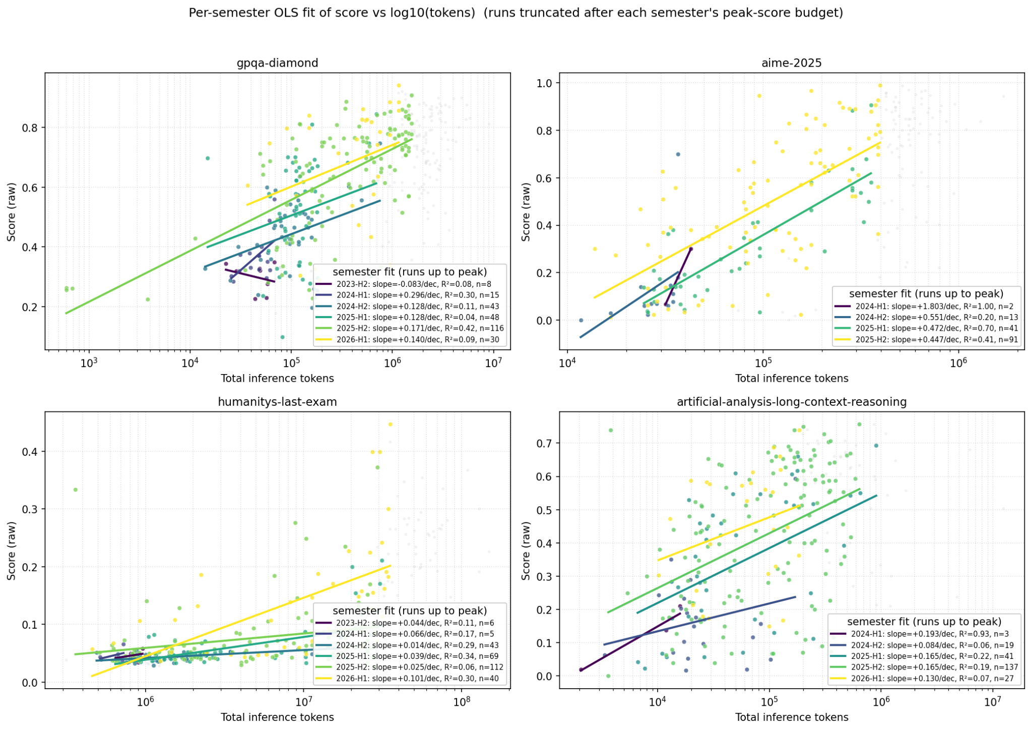
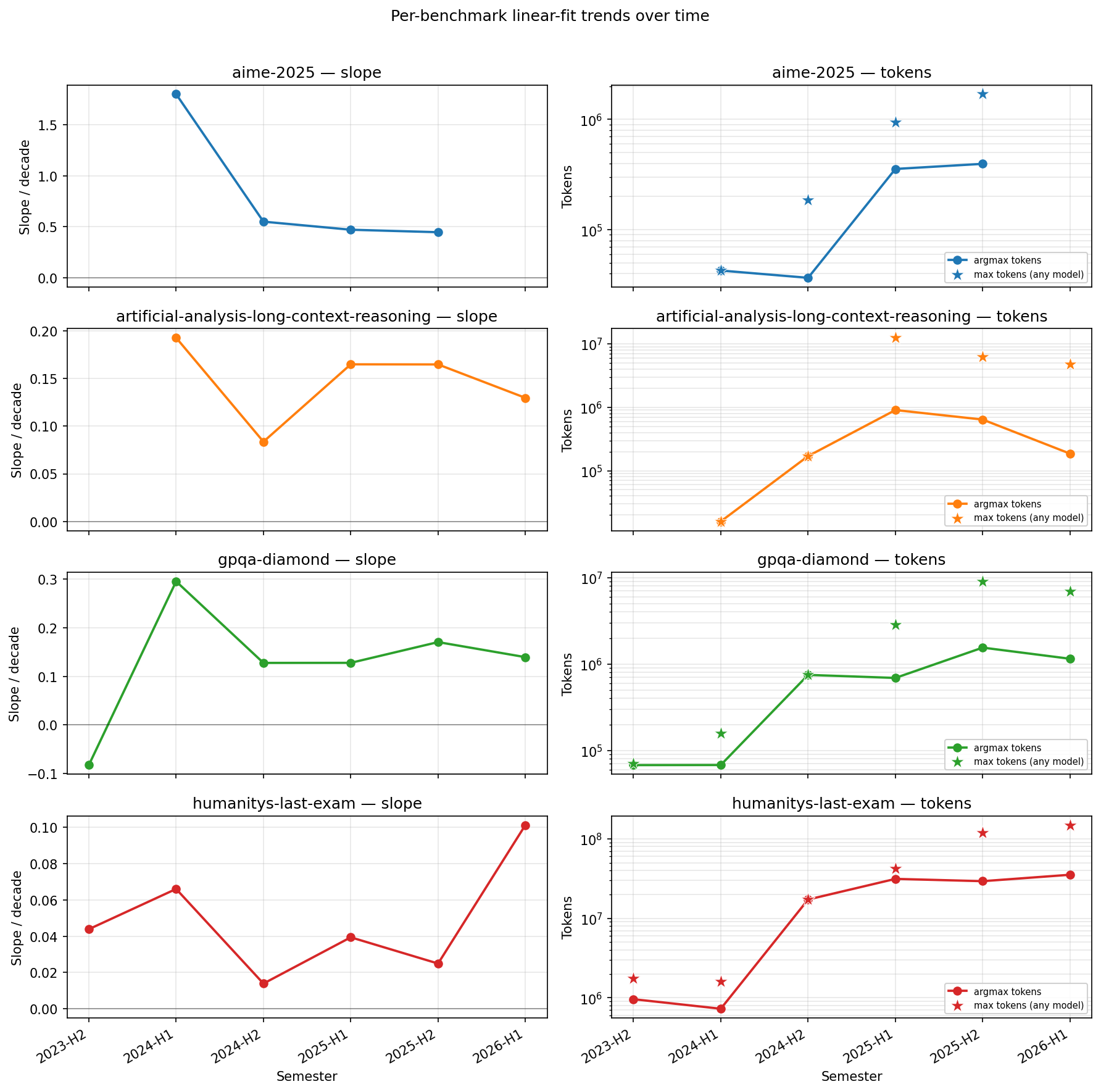
Figure 8 fits a straight line across model performance for a given inference token budget. As we saw previously, model performance starts to decrease after a certain number of inference tokens is reached, so I decided to leave out models whose performance was lower than the peak score while using more inference tokens. This is fine since the idea is to see general trends in the rates at which models are able to use tokens to gain capabilities. The image does not show a general trend across semesters in the rates at which models increase performance as they scale inference token usage.

To be more confident, Figure 9 plots the rate at which score increases per additional inference token (the slope from Figure 8) for every semester. We can see on the left column that changes in the slope are mixed across benchmarks. AIME shows a consistent deceleration, while the others show a mixed result, with rates fluctuating over time. All benchmarks show a decline between the first and second semester of 2024. This is an interesting result given that the first reasoning model was released in the second semester of 2024. The slopes are also relatively more stable and have less variation in the second semester of 2024 and all of 2025. This seems to be the case for AIME, GPQA and HLE. This is due to the fact that we have more data for those time periods.

We can also look at the maximum number of tokens that can be used before getting diminishing returns. This is important because it means that models are able to extract capability gains for longer periods. This is plotted on the right column of the image below. We can see that, over time, models are able to scale their inference tokens for longer before plateauing or decreasing in performance, with AALCR being the only significant exception. The stars represent the maximum number of tokens used by any model for each period. For most periods, using the most amount of inference tokens did not mean obtaining the highest score, showing that inference tokens were scaled beyond the point after which decreasing returns begin to appear. Some benchmarks monotonically increased the maximum amount of inference tokens used per semester (AIME, HLE) while others showed a slight decline (AALCR, GPQA).

Inference scaling for training more capable models

Ord’s second argument might be more worrisome for training compute thresholds. He describes a recursive self-improvement loop in which models leverage inference scaling to produce high-quality synthetic data, which is then used to train a superior model of comparable scale. This idea, also called iterated distillation and amplification, is similar to the mechanism behind Alpha Go Zero, and was independently discovered by Anthony et al. and, in the context of AI Safety, by Cristiano. While the exact mechanism of how this could work is still uncertain, we can still look at current trends to understand the role of inference scaling in the training process.

Models are being optimized for inference

Since generating vast amounts of synthetic training data could be expensive (especially for high quality data requiring long chains of thought and inference scaling), we care about cheap and efficient inference. Fast and cheap inference is driven by several factors, including hardware improvements and algorithmic efficiency gains.

Beyond these, AI labs can also optimize models for inference-heavy tasks. The main way to do this is by reducing the model size. Smaller models make inference faster and cheaper and are easier to use for researchers and developers with limited GPU resources. One approach for reducing model size is pruning, which involves the periodical removal of irrelevant weights during training. Another approach, explained by de Vries, is varying the scaling policy. For a given training compute budget, AI labs can decide to overtrain a smaller model on more tokens than Chinchilla scaling laws would suggest.

The graph below shows this dynamic. On the left column, I compare the actual number of parameters against the optimal number of parameters each model should have according to Chinchilla scaling laws. Over time, it is clear that models are getting smaller against their Chinchilla optimal number of parameters. The fitted line suggests models shrink by about ×0.58 per year, or roughly half every 15 months. On the right side of the graph is the number of tokens used to train each model. The trend is also clear. Models are being increasingly trained with more tokens than Chinchilla optimality would suggest.

‍

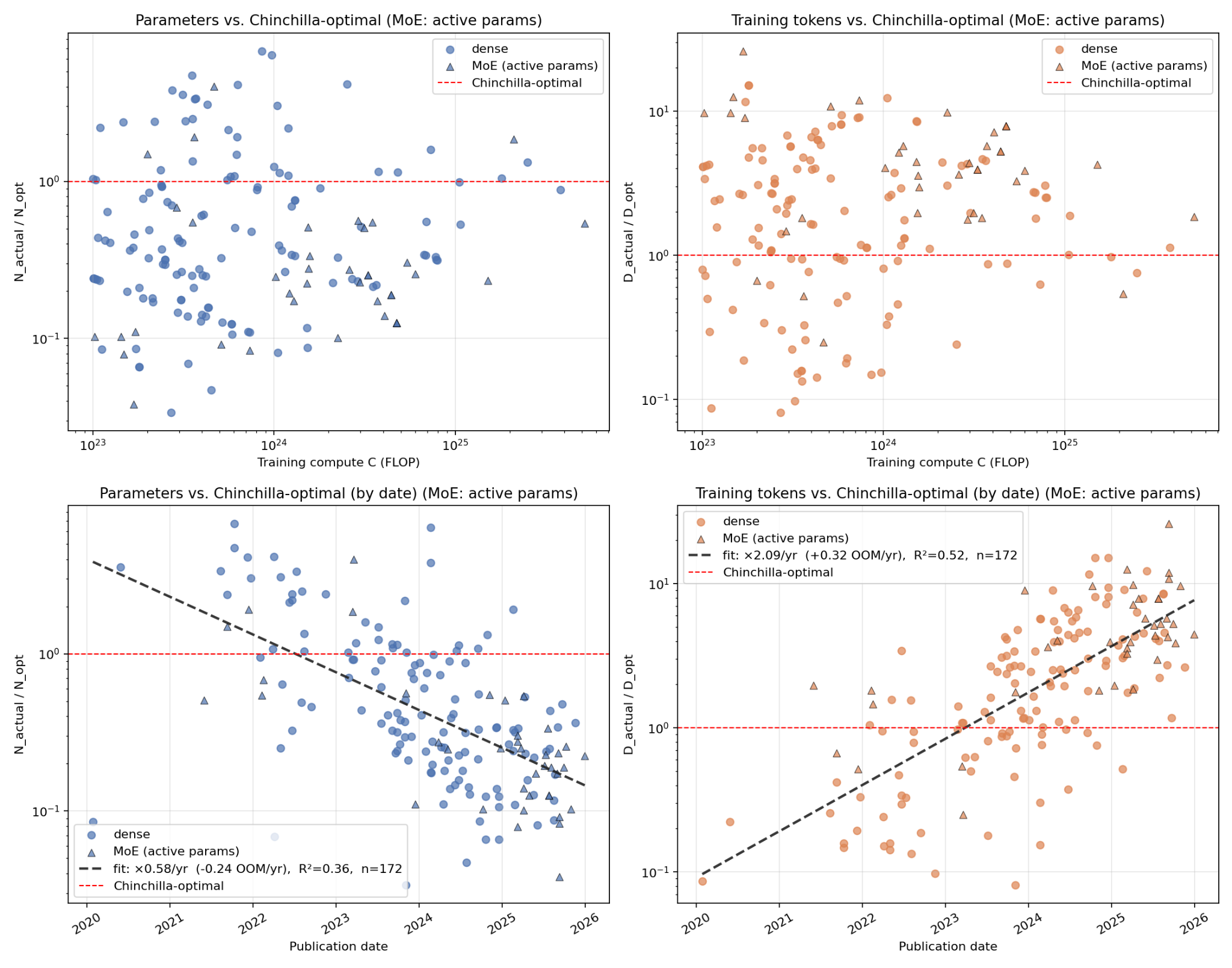
An interesting question is how much smaller can models get. Sardana et al were able to shrink models down to 10k tokens per parameter without an impact on loss while De Vries estimates that the critical model size is around 30% of the Chinchilla optimal model. Huang et al. found a critical size below which models cannot learn the rare and complex tasks in the tail of the data distribution even with unlimited data, because the tasks that dominate the training data consume the model's limited capacity, leaving too little for the rare ones.

Inference costs are falling

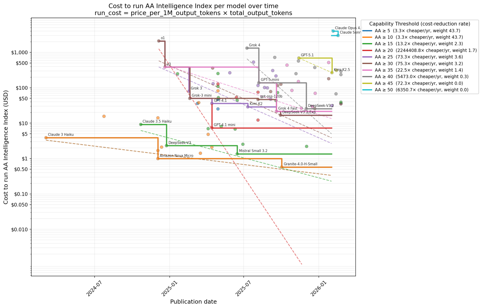
Shrinking model sizes, hardware efficiency gains, and other sources of algorithmic progress have together driven inference prices down sharply. The estimates of the rates at which prices decline vary across benchmarks. For example, Epoch estimated that prices fall by between 9x and 900x per year, with a median of 50x. In his analysis, Scher estimated that the cost per 1M tokens is falling at around 82x per year. He also mentions that per-token costs is not as relevant as the cost to run benchmarks (measured as the cost per token * number of tokens). I agree because, as seen in previous graphs, some models are more token efficient than others. I decided to expand his analysis and calculate the cost to run the Artificial Analysis Intelligence Index (AAII), since they publish the number of tokens used to run this benchmark. The result is a tiny bit more conservative than the per-token rate, with the cost to run AAII falling at a median rate of 73x per year.

Beyond the median, I also calculated a weighted average of the slopes, where each weight corresponds to the inverse variance of the slope (1/SE2) normalized to sum to 100. With these parameters, the cost to run AAII falls at a rate of around 32,000x per year. As we can see in the graph below, this is likely due to the AA >= 20 threshold slope being an outlier. This is because the o1 model, the first reasoning model with a really high cost per token and a high token usage, heavily skews the slope. If we exclude the entire AA >= 20 threshold, the weighted slope falls at a rate of 27x per year. These results highlight the high variability associated with these estimations.

Implications for AI Governance and Compute Thresholds

It remains unclear how training compute shapes both the rate at which a model improves with more inference tokens and the point at which further tokens no longer help. What does appear strong is the relationship between training compute and token efficiency, meaning the number of tokens a model needs to reach a given performance level. This dependence between inference scaling and training compute suggests that training compute thresholds remain a viable governance instrument.

Empirical analysis shows that saving 1 OOM of training compute costs roughly 1.4 OOM of inference compute, consistent with Villalobos and Atkinson's estimates. Diminishing returns also persist across all observed release periods, with no benchmark showing the inflection toward unbounded inference scaling. If this trend holds, then for a given amount of training compute there is an upper limit on the capability gains achievable through inference scaling. Pushing past that limit would require more training compute. While these two observations slightly undermine Ord's worry that a 10^24 FLOP model could be inference-scaled into a 10^27 effective-FLOP model, the effect on capabilities should not be discounted. Training compute thresholds should still take into account the possible jump in capabilities stemming from inference scaling.

Task dependence narrows the threat surface further. Inference scaling substitutes for training compute most effectively on harder, longer-horizon tasks, where larger models gain more capability per inference token, while smaller models struggle. This suggests that model size is an important variable beyond training compute thresholds, since a model's size shapes its ability to benefit from inference scaling.

However, the relationship between training and inference compute is not guaranteed. Slopes are steepening on some benchmarks and argmax tokens are rising, meaning models extract more capability per inference token and sustain gains for longer before plateauing.

On Ord's second argument regarding iterated distillation and amplification, the evidence is more circumstantial. Models are consistently smaller and more overtrained than Chinchilla-optimal, which is consistent with labs optimizing for cheap inference, exactly the configuration that synthetic data pipelines require. Inference costs are also falling sharply, 73x per year on AAII. Together these trends mean the marginal cost of producing high-quality reasoning traces for post-training is collapsing. Whether labs are actually closing an iterated distillation and amplification loop is not directly observable from this data, but the preconditions are clearly in place.

Based on this data, the evidence that inference scaling will inevitably erode training compute thresholds is mixed. Ord's first argument, on scaling inference on deployed models, is weakened, while his second argument, on iterated distillation and amplification, remains a challenge. Training compute thresholds are still useful, but inference scaling trends are worth monitoring so the thresholds can be adjusted as needed. The dependence of inference scaling on training compute should also be tracked continuously, since any decoupling would undermine the assumption that a model's training compute bounds its eventual capabilities.

Limitations

The dominant limitation of this analysis is data scarcity. Public evaluation runs are sparse when sliced by training compute, inference tokens, and release period simultaneously, which prevents finer-grained analysis of the two questions that matter most for governance. The first of these questions is whether diminishing returns are themselves changing over time. The current analysis shows that diminishing returns persist across all observed periods, but the data is too thin to tell whether the rate of diminishing returns is softening within a fixed training compute band. The second is whether the training-inference trade-off ratio is shifting. The 1.4 OOM trade-off observed here is a snapshot, and tracking how this ratio evolves over time requires repeated measurements across the same training compute bands, which the current dataset does not support.

Several smaller limitations are downstream of this same scarcity. The benchmark suite is narrow and skewed toward STEM and verifiable tasks, since these are the benchmarks with enough public evaluation runs to support the analysis. Training compute values are estimates rather than disclosed figures for most closed models, with error bars wide enough to affect the trade-off ratio. Inference compute is approximated by inference tokens which loses precision across architectures with different per-token FLOP costs.

Future work

My analysis shows that a single benchmark run yields diminishing returns as the token budget grows, but it does not capture the effect of repeated sampling and filtering. This form of inference scaling deserves further study.

Another open question is how much inference scaling should factor into estimates of safe training compute thresholds. Current trade-off estimates provide a good intuition, but more work could be done in the context of MIRI’s pre-training and post-training compute thresholds.

‍

Appendix

For each of the ten graphs above, I list the source script, the input datasets it reads, the processing steps it applies, and the output CSV that holds the underlying numbers. Graphs 1–9 live in this repo (feruiloba/miri-fellowship-inference-scaling) on the master branch. Graph 10 lives in the sibling repo (feruiloba/miri-fellowship-alg-progress) on the main branch.

‍

Shared inputs

Most graphs read from a small set of curated CSVs under data/:

‍

aa_evaluations_combined.csv

per-benchmark evaluation runs scraped from Artificial Analysis. One row per (model_slug, benchmark) with score_raw, total_output_tokens, and related fields. This is the dominant data source for the inference-token analyses.

artificial_analysis_llm_stats.csv

per-slug model metadata, used here for release_date

aa_output_tokens.csv

per-model token counts used to compute AA-Index.

epoch_all_ai_models.csv

Epoch AI's curated model table. Source of Training compute (FLOP) for closed-weights models.

merged_datasets.csv

internal join of Epoch + AA tables. Provides Training compute (FLOP), Publication date, parameter counts, and an is_moe flag for the Chinchilla analysis and the iso-capability plot

‍

Two graphs are produced by scripts that read derived CSVs written by other scripts in this repo; those producer-consumer chains are called out explicitly below.

‍

1. Inference scaling has diminishing returns

Graph: top10_per_token_band.png

Script: top10_per_token_band.py

Table: top10_per_token_band.csv

Inputs: aa_evaluations_combined.csv, artificial_analysis_llm_stats.csv (release dates for the colour scale).

‍

Method: For each of four target benchmarks (GPQA-Diamond, AIME 2025, Humanity's Last Exam, AA long-context-reasoning), filter to runs with a valid positive total_output_tokens and score_raw. Bucket runs into 8 log-spaced inference-token bands spanning the observed token range. Within each band, take the top-10 runs by score_raw and compute their mean and standard error. Plot one panel per benchmark: a single aggregate line (top-10 mean with ±SEM whiskers) overlaid on a scatter of every run coloured by release date. The CSV has one row per (benchmark, band) with n, mean_top10_score, sem, and the band bounds.

‍

2. Iso-capability bands by training compute

Graph: top10_grouped_by_training_compute_band.png

Script: top10_grouped_by_training_compute_band.py

Table: top10_grouped_by_training_compute_band.csv

Inputs: aa_evaluations_combined.csv plus epoch_all_ai_models.csv for Training compute (FLOP). Slugs are matched against the Epoch table with a fallback that strips parenthesised suffixes from model names.

‍

Method: Same skeleton as graph 1 (4 benchmarks, 8 log-spaced inference-token bands, top-10 mean per band), but runs are first grouped into half-decade training-compute bands with edges at every 0.5 dex from 10²² to 10²⁷ FLOP. Each compute band becomes a separate viridis-coloured curve so the L-shape across (training compute × inference tokens) is visible. For GPQA-Diamond the script also draws a horizontal reference line at score = 0.7 and annotates, for each curve, the interpolated token count at which it crosses that line — this is the source of the "1.4 OOM trade-off" figure quoted in the writeup. MoE models are included. The CSV has one row per (benchmark, compute_band, token_band) cell.

‍

3. Iso-capability frontier (training FLOPs vs inference tokens)

Graph: train_flops_vs_inference_tokens_top5_score.png

Script: train_flops_vs_inference_tokens_top5_score.py

Table: train_flops_vs_inference_tokens_top5_score.csv

Inputs: aa_evaluations_combined.csv joined to merged_datasets.csv on AA_slug for Training compute (FLOP).

‍

Method: Per benchmark, restrict to the top-5 scoring runs at each combination of training-compute and inference-token band. The chart plots training FLOP on the X axis vs inference tokens on the Y axis, with marker colour encoding the score and contours implied by the top-5 mean per cell — this directly visualises the trade-off frontier the writeup refers to as "L-shaped". The CSV records each (training compute band, inference token band, benchmark, top-5 score).

‍

4. Inference scaling is domain-dependent (gpt-oss case study)

Graph: gpt_oss_effort_comparison.png

Script: gpt_oss_effort_comparison.py

Table: No CSV written by this script. The underlying slope numbers quoted in the writeup come from the table produced by graph 5 (gpt_oss_training_inference_tradeoff.csv, columns beta_20, beta_120).

Inputs: aa_evaluations_combined.csv, restricted to the four gpt-oss slugs: gpt-oss-20b, gpt-oss-20b-low, gpt-oss-120b, gpt-oss-120b-low.

‍

Method: For every benchmark that has both effort levels for both model sizes (low/high effort × 20b/120b), draw a 2-point line per model in (log10 total_output_tokens, score_raw) space. The two lines per panel directly visualise per-model inference-token slopes; the writeup compares them visually for scicode vs tau2-bench.

‍

5. Training-vs-inference substitution rate (gpt-oss)

Graph: gpt_oss_training_inference_tradeoff.png

Script: gpt_oss_training_inference_tradeoff.py

Table: gpt_oss_training_inference_tradeoff.csv

Inputs: aa_evaluations_combined.csv, same gpt-oss slug filter as graph 4. Training-compute ratio hard-coded as log10(4.94e24 / 5.49e23) ≈ 0.954 ≈ 9× (from Epoch's training-compute estimates for the two gpt-oss models).

‍

Method: For each benchmark with all four corners (size × effort) present, compute four finite-difference slopes from the 2×2 grid:

‍

α_low = (s(120,low) − s(20,low)) / log10(9) — ∂score/∂log(C_train) at low effort

α_high = (s(120,high) − s(20,high)) / log10(9) — ∂score/∂log(C_train) at high effort

β_20 = (s(20,high) − s(20,low)) / Δlog(tokens_20b) — ∂score/∂log(C_inf) at 20b

β_120 = (s(120,high) − s(120,low)) / Δlog(tokens_120b) — ∂score/∂log(C_inf) at 120b

The chart shows the inference-slope ratio β_120 / β_20 as a horizontal bar per benchmark. Bars > 1 indicate the bigger model gains more per token; bars < 1 indicate the smaller model uses extra thinking more productively. The writeup quotes the 5.15× ratio for scicode straight from this CSV (r_LL/r_UR and the β columns).

‍

6. Diminishing returns over time

Graph: top10_grouped_by_release_period.png

Script: top10_grouped_by_release_period.py

Table: top10_grouped_by_release_period.csv

Inputs: aa_evaluations_combined.csv joined to artificial_analysis_llm_stats.csv on slug for release_date.

‍

Method: Same template as graph 1 (4 benchmarks, 8 log-spaced inference-token bands, top-10 mean per band), but runs are grouped by 6-month release period (YYYY-H1 / YYYY-H2). Each release period becomes a viridis-coloured curve. Cells with n < 4 are dropped, and periods with fewer than 5 total runs are excluded entirely. The chart shows the curves shifting upward over time (capability per token improving) while still bending (diminishing returns persisting). One CSV row per (benchmark, period, token_band).

‍

7. Per-semester linear fits

Graph: linear_fits_by_release_semester.png

Script: linear_fits_by_release_semester.py

Table: linear_fits_by_release_semester.csv

Inputs: aa_evaluations_combined.csv joined to artificial_analysis_llm_stats.csv for release dates.

‍

Method: Same per-cell aggregation as graph 6 (8 log-spaced bands, top-10 per cell, per semester). On top of those cell means, fit an OLS line score = a + b · log10(tokens) per (benchmark, semester). Plot the fitted lines (viridis by semester) over the top-K cell scatter. The CSV records slope_per_decade, intercept, r2, n_fit_points, period, and benchmark — one row per (benchmark, semester). This CSV is the input to graph 8.

‍

8. Slope and argmax-token trends across semesters

Graph: semester_fit_trends.png

Script: semester_fit_trends.py

Table: semester_fit_trends.csv

Inputs: linear_fits_by_release_semester.csv (the table from graph 7) plus aa_evaluations_combined.csv and artificial_analysis_llm_stats.csv for the argmax-tokens computation.

‍

Method: Two columns per benchmark row: the left column plots slope_per_decade over semester time (linear y-axis, with slope = 0 reference line); the right column plots argmax-tokens per (benchmark, semester) on a log scale, where argmax-tokens is the total_output_tokens of the single highest-scoring run in that cell. The CSV adds argmax_tokens, argmax_score, argmax_model, delta_slope, delta_intercept, and argmax_token_ratio (period-over- period change) to the per-semester fit table. This is the chart the writeup uses to argue "slopes are steepening and argmax tokens are rising" across most benchmarks.

‍

9. Chinchilla optimality drift (parameters and training tokens)

Graph: chinchilla_param_token_vs_optimal_moe_active.png

Script: chinchilla_param_token_vs_optimal_moe_active.py (uses helpers from src/chinchilla_analysis/_chinchilla.py)

Table: chinchilla_param_token_vs_optimal_moe_active.csv

Inputs: merged_datasets.csv (read by _chinchilla.py). Provides Training compute (FLOP), Publication date, parameter counts, training tokens, and an is_moe flag.

‍

Method: For each model with known training compute, parameters, and training tokens, compute the Chinchilla-optimal N_opt, D_opt from C = 6 · N · D and the Hoffmann et al. exponents, then take the ratios N_actual / N_opt and D_actual / D_opt. For MoE models, N_actual is replaced by N_active = C / (6 · D_actual) so the model is compared at its inference-time parameter count rather than its total parameter count. The chart is a 2×2 grid: top row plots the two ratios against training compute (log-log); bottom row plots them against publication date, with an OLS fit drawn on the date panels. The "×0.58 per year" figure quoted in the writeup is the 10**slope factor from the parameter-ratio-vs-date fit. The CSV is one row per model with the input columns plus the derived ratios and an arch column (dense or moe_active).

‍

10. Run-cost frontier (sibling repo)

Graph: run_cost_frontier.png

Script: 03_cost_to_run_catchup_by_tokens.py

Table:  run_cost_frontier_table.csv

Inputs:

merged_datasets.csv (publication dates and AA-Index per model)

aa_output_tokens.csv (per-model token counts for running AAII)

‍

Method: Join the two tables on AA slug. For each model, compute run_cost_usd = output_token_price · total_output_tokens — i.e. the dollar cost to run the full AAII benchmark using that model's token budget at its API price. For each capability threshold (an AA-Index level), restrict to models above that threshold, sort by publication date, take the cumulative minimum of run_cost_usd to get the Pareto frontier of cheapest-yet-released-most-capable models, then fit log10(run_cost) = slope · days + intercept on the frontier points to derive an annual catch-up factor. The "73× per year" figure quoted in the writeup is 10**(365·slope) from that fit at the AAII threshold. The CSV records, per threshold, the catch-up slope, the implied yearly factor, and the frontier point list.

‍